Assembling a mitochondrion genome with the ORGanelle ASeMbler ¶

We are presenting here a simple case desmonstrating how to assemble a mitochondrial genome from a genome skimming dataset. The dataset used for this tutorial corresponds to a simulated datased presenting no difficulty for its assembling. The aims of this tutorial is only to guide you during your first steps with the ORGanelle ASeMbler.

The dataset is composed of two files

a forward fastq file : papi_R1.fastq.gz

a reverse fastq file : papi_R2.fastq.gz

Step 1 : indexing the reads¶

To assemble a genome from sequence reads, you need first to index them. This step allows an efficient access to the reads during the assembling process. The organelle assembler is optimized for running with paired end Illumina reads. It can also works, but less efficiently, with single reads, and 454 or Ion Torrent reads.

Considering two fastq files papi_R1.fastq.gz and papi_R2.fastq.gz containing respectively the forward and the reverse reads of the paired reads, to build the index named butterfly from a UNIX terminal you have to run the oa index command:

> oa index --estimate-length=0.9 butterfly papi_R1.fastq.gz papi_R2.fastq.gz

This command produce the following screen output

2018-12-12 11:30:39,337 [INFO ]  orgasmi -o butterfly.odx/index /var/folders/84/_g1lrhc11x170szbh74py3580000gn/T/tmp73yausim/forward-pg1ky01i /var/folders/84/_g1lrhc11x170szbh74py3580000gn/T/tmp73yausim/reverse-mq8tq3j2
2018-12-12 11:30:39,337 [INFO ]  Starting indexing...
2018-12-12 11:30:39,341 [INFO ]  Forward tmp file : /var/folders/84/_g1lrhc11x170szbh74py3580000gn/T/tmp73yausim/forward-pg1ky01i
2018-12-12 11:30:39,341 [INFO ]  Reverse tmp file : /var/folders/84/_g1lrhc11x170szbh74py3580000gn/T/tmp73yausim/reverse-mq8tq3j2

Reading sequence reads...

2018-12-12 11:30:39,347 [INFO ]  Selecting the best length to keep 90.0% of the reads.

2018-12-12 11:30:39,356 [INFO ]     Minimum length set to 0bp

2018-12-12 11:30:39,357 [INFO ]  Soft clipping bad quality regions (below 10).

2018-12-12 11:30:39,357 [INFO ]  Select the longest region containing only [A,C,G,T]

2018-12-12 11:30:39,358 [INFO ]  Two files pair-end data
Read length estimate [   40960] speed :  84518.4 reads/s

2018-12-12 11:30:39,908 [INFO ]  Indexing length estimated to : 100bp
Read length adjusted to 99
maximum reads : 55555555
    94742 sequences read

Sorting reads...

    94742 sequences sorted

Writing sorted sequence reads...

    94742 sequences read

Writing sequence pairing data...

Done.

Reading indexed sequence reads...

    94742 sequences read

Sorting reads...

    94742 sequences sorted

Writing sequence suffix index...

Done.

Writing global data...

Done.
2018-12-12 11:30:42,692 [INFO ]  Done.
2018-12-12 11:30:42,692 [INFO ]      47371 reads pairs processed
2018-12-12 11:30:42,692 [INFO ]          0 reads pairs soft trimmed on a quality of 10
2018-12-12 11:30:42,692 [INFO ]          0 reads pairs clipped for not [A,C,G,T] bases

Loading global data...

Done.

Reading indexed sequence reads...

    94742 sequences read

Reading indexed pair data...

Done.

Loading reverse index...

Done.

Indexing reverse complement sequences ...

Fast indexing forward reads...

Fast indexing reverse reads...

Done.
2018-12-12 11:30:42,697 [INFO ]  Count of indexed reads: 94742
Deleting tmp file : /var/folders/84/_g1lrhc11x170szbh74py3580000gn/T/tmp73yausim/reverse-mq8tq3j2
Deleting tmp file : /var/folders/84/_g1lrhc11x170szbh74py3580000gn/T/tmp73yausim/forward-pg1ky01i
Deleting tmp directory : /var/folders/84/_g1lrhc11x170szbh74py3580000gn/T/tmp73yausim

the oa index command is able to manage with compressed read files :

by gzip (file name ending by .gz)

by bzip2 (file name ending by .bz2)

and to estimed the better indexing length to use –estimate-length option.

By using the following Unix command you can observe that the oa index produced a directory named butterfly.odx. It contains the indexed reads. The two fastQ files will not anymore used.

> ls -l
    total 4704
    drwxr-xr-x  6 coissac  staff      192 12 déc 11:30 butterfly.odx
    -rw-r--r--  1 coissac  staff  1201837 12 déc 11:30 papi_R1.fastq.gz
    -rw-r--r--  1 coissac  staff  1202027 12 déc 11:30 papi_R2.fastq.gz

Step 2 : Building the assembling graph¶

Now than the reads are indexed, we have to build the assembling graph. This job is done by the oa buildgraph command. This command can be launched with the following Unix command:

$ oa buildgraph --probes protMitoMachaon butterfly butterfly.mito

This ask for assembling the reads indexed in the butterfly index, using the internal seed sequences named protMitoMachaon and constituted by the set of protein sequences of the machaon mitochondrial genome. The results will be stored in a directory named butterfly.mito.oas

2018-12-12 12:08:46,198 [INFO ]  Building De Bruijn Graph
2018-12-12 12:08:46,199 [INFO ]  Minimum overlap between read: 50

The first lines printed recall the current operation and the minimum length of the overlap between two reads required during the assembling process.

Then the index is loaded in memory. For this tutorial we are assembling a simulated dataset containing only 94742 sequences. A true dataset contains usualy several millons of reads.

Loading global data...

Done.

Reading indexed sequence reads...

    94742 sequences read

Reading indexed pair data...

Done.

Loading reverse index...

Done.

Indexing reverse complement sequences ...

Fast indexing forward reads...

Fast indexing reverse reads...

Done.

The assembler then load a set of external data and the protMitoMachaon seed set requested by the –seeds option.

2018-12-12 12:08:46,203 [INFO ]  Load 3' adapter internal dataset : adapt3ILLUMINA
2018-12-12 12:08:46,204 [INFO ]  Load 5' adapter internal dataset : adapt5ILLUMINA
2018-12-12 12:08:46,204 [INFO ]  Load probe internal dataset : protMitoMachaon

According to the global assembling algorithm the first step of the assembling constists in looking for the reads presenting sequence similaritiy with seed sequences.

2018-12-12 12:08:46,204 [INFO ]  No previous matches loaded
2018-12-12 12:08:46,204 [INFO ]  Running probes matching against reads...
2018-12-12 12:08:46,204 [INFO ]      -> probe set: protMitoMachaon
2018-12-12 12:08:46,205 [INFO ]  Matching against protein probes
Building Aho-Corasick automata 100.0 % |##################################################/] remain : 00:00:00
2018-12-12 12:08:54,402 [INFO ]  Minimum word matches = 16
  98.5 % |#################################################\ ] remain : 00:00:00
2018-12-12 12:08:56,091 [INFO ]  ==> 10724 matches
2018-12-12 12:08:56,096 [INFO ]  Match list :
2018-12-12 12:08:56,098 [INFO ]       nd3        :  1497 (422.2x)
2018-12-12 12:08:56,098 [INFO ]       nd4L       :   981 (337.2x)
2018-12-12 12:08:56,099 [INFO ]       atp6       :  1765 (257.7x)
2018-12-12 12:08:56,099 [INFO ]       cox3       :  1615 (203.4x)
2018-12-12 12:08:56,099 [INFO ]       nd1        :  1679 (177.6x)
2018-12-12 12:08:56,099 [INFO ]       cytB       :  1772 (153.1x)
2018-12-12 12:08:56,099 [INFO ]       nd6        :   714 (133.1x)
2018-12-12 12:08:56,099 [INFO ]       cox1       :  1586 (102.6x)
2018-12-12 12:08:56,099 [INFO ]       nd4        :   731 ( 54.1x)
2018-12-12 12:08:56,099 [INFO ]       cox2       :   222 ( 32.3x)
2018-12-12 12:08:56,099 [INFO ]       atp8       :     5 (  3.0x)
2018-12-12 12:08:56,099 [INFO ]       nd5        :    39 (  2.2x)
2018-12-12 12:08:56,099 [INFO ]       nd2        :     2 (  0.2x)
2018-12-12 12:08:56,099 [INFO ]  No previous assembling
2018-12-12 12:08:56,099 [INFO ]  Starting a new assembling
2018-12-12 12:08:56,100 [INFO ]  Coverage estimated from probe matches at : 422

In that case, 10724 matches where identified and they belong several genes as shown by the printed table. This table allows also to make a first estimation of the sequencing coverage (422x). This coverage estimation is important because it allows to set the assembling parametters. The estimation realized from matches is higly approximative. To make a better estimate, 15kb of sequences are assembled following this first estimation.

2018-12-12 12:08:56,100 [INFO ]  Assembling of 15000 pb for estimating actual coverage
2018-12-12 12:08:56,127 [INFO ]  0 bp [ 0.0% fake reads; Stack size:    10723 /  -1.00 0  Gene: nd2
2018-12-12 12:09:08,275 [INFO ]  10000 bp [ 0.0% fake reads; Stack size:    10714 /   0.00 0  Gene: cox2
| : 14989 bp [ 0.0% fake reads; Stack size:    10714 /   0.00 0  Gene: cox2
Compacting graph 100.0 % |#################################################- ] remain : 00:00:00
2018-12-12 12:09:15,719 [INFO ]  Minimum stem coverage = 393

Deleting terminal branches

Compacting graph 100.0 % |#################################################- ] remain : 00:00:00
2018-12-12 12:09:15,955 [INFO ]  Minimum stem coverage = 393
2018-12-12 12:09:15,956 [INFO ]  Dead branch length set to : 10 bp

Compacting graph 100.0 % |#################################################- ] remain : 00:00:00
2018-12-12 12:09:16,312 [INFO ]  Minimum stem coverage = 393
2018-12-12 12:09:16,347 [INFO ]  coverage estimated : 393x based on 14999 bp (minread: 64)

This allows to get a second coverage estimate (here 393x) which is far most precise. The true assembling stage can now be run.

2018-12-12 12:09:16,374 [INFO ]  Starting the assembling
2018-12-12 12:09:16,374 [INFO ]  0 bp
[ 0.0% fake reads; Stack size:    10723 /  -1.00 0  Gene: nd2
2018-12-12 12:09:29,995 [INFO ]  10000 bp
[ 0.0% fake reads; Stack size:    10714 /   0.00 0  Gene: cox2
| : 15185 bp [ 0.0% fake reads; Stack size:      109 /  -1.00 0  Gene: nd3

In our case it leads to the assembling of 15185 bp in less of a minute.

Following the assembling a cleaning step is run to simplifly the assembling graph by removing allow the aborted paths mainly created by sequencing errors and nuclear copies of some part of the mitochondrial genome.

Compacting graph 100.0 % |##################################################-] remain : 00:00:00
2018-12-12 12:09:39,503 [INFO ]  Minimum stem coverage = 393

Deleting terminal branches
2018-12-12 12:09:39,705 [INFO ]   Circle :  15185 bp coverage :    393x
Compacting graph  50.0 % |#########################/                         ] remain : 00:00:002
2018-12-12 12:09:39,864 [INFO ]       Dead branch length setup to : 10 bp
Compacting graph 100.0 % |##################################################-] remain : 00:00:00
2018-12-12 12:09:40,400 [INFO ]  Minimum stem coverage = 393

Following this cleaning a last estimate of the coverage is done. Moreover the assembler estimates the insert size and the variance of this size. This estimate is computed from the relative positions of the pair-end reads in the assembling graph.

2018-12-12 12:09:40,449 [INFO ]  coverage estimated : 393 based on 15185 bp
2018-12-12 12:09:40,660 [INFO ]   Circle :  15185 bp coverage :    393x
Compacting graph  50.0 % |#########################/                         ] remain : 00:00:002
2018-12-12 12:09:40,792 [INFO ]   Circle :  15185 bp coverage :    393x
Compacting graph 100.0 % |##################################################-] remain : 00:00:00
2018-12-12 12:09:40,803 [INFO ]  Minimum stem coverage = 393
2018-12-12 12:09:40,933 [INFO ]  Fragment length estimated : 100.000000 pb (sd: 0.000000)

Because of our artificial dataset, the insert size is precisely 100bp and the standard deviation is null.

When the sequence coverage is too low and/or when some low complexity sequences (micro-satellite) are present into the genome the assembler is not able to produce the complete sequence as a single contig.

To save these assembling a gap-filling step is systematically run for trying to reduce as much as possible the number of contigs. Usually the ORGanelle ASeMbler finished after this step with a single contig.

Compacting graph 100.0 % |##################################################-] remain : 00:00:00
2018-12-12 12:09:42,822 [INFO ]  Minimum stem coverage = 393
Deleting terminal branches
2018-12-12 12:09:43,020 [INFO ]   Circle :  15185 bp coverage :    393x
Compacting graph  50.0 % |#########################/                         ] remain : 00:00:002
2018-12-12 12:09:43,228 [INFO ]   Circle :  15185 bp coverage :    393x
Compacting graph 100.0 % |##################################################-] remain : 00:00:00
2018-12-12 12:09:43,238 [INFO ]  Minimum stem coverage = 393
Dead branch length setup to : 10 bp
Remaining edges : 30370 node : 30370
#######################################################
#
# Added : 0 bp (total=15185 bp)
#
#######################################################

In our case the assembling was complete so no base-pair was added and the gap-filling procedure stop quicly.

The assembling procedure ends with a last cleaning step:

==================================================================
2018-12-12 12:09:43,534 [INFO ]   Circle :  15185 bp coverage :    393x
Compacting graph  50.0 % |#########################/                         ] remain : 00:00:00
2018-12-12 12:09:43,671 [INFO ]   Circle :  15185 bp coverage :    393x
Compacting graph 100.0 % |##################################################-] remain : 00:00:00
2018-12-12 12:09:43,694 [INFO ]  Minimum stem coverage = 393
2018-12-12 12:09:43,936 [INFO ]   Circle :  15185 bp coverage :    393x
Compacting graph  50.0 % |#########################/                         ] remain : 00:00:00
2018-12-12 12:09:44,068 [INFO ]   Circle :  15185 bp coverage :    393x
Compacting graph 100.0 % |##################################################-] remain : 00:00:00
2018-12-12 12:09:44,084 [INFO ]  Minimum stem coverage = 393

==================================================================

2018-12-12 12:09:44,239 [INFO ]  Clean dead branches
2018-12-12 12:09:44,429 [INFO ]   Circle :  15185 bp coverage :    393x
Compacting graph  50.0 % |#########################/                         ] remain : 00:00:00
2018-12-12 12:09:44,584 [INFO ]   Circle :  15185 bp coverage :    393x
Compacting graph 100.0 % |##################################################-] remain : 00:00:00
2018-12-12 12:09:44,600 [INFO ]  Minimum stem coverage = 393
2018-12-12 12:09:44,601 [INFO ]       Dead branch length setup to : 10 bp
Remaining edges : 30370 node : 30370
2018-12-12 12:09:44,908 [INFO ]   Circle :  15185 bp coverage :    393x
Compacting graph  50.0 % |#########################/                         ] remain : 00:00:00
2018-12-12 12:09:45,055 [INFO ]   Circle :  15185 bp coverage :    393x
Compacting graph 100.0 % |##################################################-] remain : 00:00:00
2018-12-12 12:09:45,074 [INFO ]  Minimum stem coverage = 393
2018-12-12 12:09:45,269 [INFO ]   Circle :  15185 bp coverage :    393x
Compacting graph  50.0 % |#########################/                         ] remain : 00:00:00
2018-12-12 12:09:45,413 [INFO ]   Circle :  15185 bp coverage :    393x
Compacting graph 100.0 % |##################################################-] remain : 00:00:00
2018-12-12 12:09:45,424 [INFO ]  Minimum stem coverage = 393
2018-12-12 12:09:45,475 [INFO ]  Clean low coverage terminal branches
2018-12-12 12:09:45,678 [INFO ]   Circle :  15185 bp coverage :    393x
Compacting graph  50.0 % |#########################/                         ] remain : 00:00:00
2018-12-12 12:09:45,832 [INFO ]   Circle :  15185 bp coverage :    393x
Compacting graph 100.0 % |##################################################-] remain : 00:00:00
2018-12-12 12:09:45,849 [INFO ]  Minimum stem coverage = 393

Deleting terminal branches

2018-12-12 12:09:45,850 [INFO ]  Clean low coverage internal branches
2018-12-12 12:09:46,034 [INFO ]   Circle :  15185 bp coverage :    393x
Compacting graph  50.0 % |#########################/                         ] remain : 00:00:002
2018-12-12 12:09:46,184 [INFO ]   Circle :  15185 bp coverage :    393x
Compacting graph 100.0 % |##################################################-] remain : 00:00:00
2018-12-12 12:09:46,203 [INFO ]  Minimum stem coverage = 393

Deleting terminal branches

Deleting internal branches

2018-12-12 12:09:46,204 [INFO ]  Saving the assembling graph
2018-12-12 12:09:46,869 [INFO ]   Circle :  15185 bp coverage :    393x
Compacting graph  50.0 % |#########################/                         ] remain : 00:00:00
2018-12-12 12:09:47,001 [INFO ]   Circle :  15185 bp coverage :    393x
Compacting graph 100.0 % |##################################################-] remain : 00:00:00
2018-12-12 12:09:47,020 [INFO ]  Minimum stem coverage = 393

And the scaffolding of the contigs if several of them persist after the gap-filling procedure.

2018-12-12 12:09:47,022 [INFO ]  Scaffold the assembly
2018-12-12 12:09:47,227 [INFO ]   Circle :  15185 bp coverage :    393x
Compacting graph  50.0 % |#########################/                         ] remain : 00:00:00
2018-12-12 12:09:47,362 [INFO ]   Circle :  15185 bp coverage :    393x
Compacting graph 100.0 % |##################################################-] remain : 00:00:00
2018-12-12 12:09:47,382 [INFO ]  Minimum stem coverage = 393

At this step asking for the listing of the current directory

> ls -l

shows that a new directory named butterfly.mito.oas were created. It contains the result of the assembly

total 4704
drwxr-xr-x  7 coissac  staff      224 12 déc 12:09 butterfly.mito.oas
drwxr-xr-x  6 coissac  staff      192 12 déc 11:30 butterfly.odx
-rw-r--r--  1 coissac  staff  1201837 12 déc 11:30 papi_R1.fastq.gz
-rw-r--r--  1 coissac  staff  1202027 12 déc 11:30 papi_R2.fastq.gz

You can have an idea of your assembly by generating a simplified graph showing the résult of your assembling.

> oa graph --gml butterfly.mito > butterfly.mito.gml

The butterfly.mito.gml generated file contains a simpliflied graph representation of the assembly. It can be visualized using any graph visualisation tools accepting the Graph Modeling Language (GML) format. For this purpose we are usualy using the Yed program.

The graph files are produced for the user convinience and they are not reuse latter by the assembler.

Step 3 : unfolding the graph to get the sequence¶

The last step required to get the sequence of the mitochondrial genome is to extract the sequence from the graph. This operation corresponds to find an optimal path in the graph. This linear path is a description of the sequence.

The oa unfold command realizes this operation and produces as final result a fasta file containing the sequence of the assembled genome.

> oa unfold butterfly butterfly.mito > butterfly.mito.fasta

The first outputs of the oa unfold command are similar to those produced by the oa buildgraph command presenting the loading of the sequence index and of the seed reads identified by the oa buildgraph command.

Loading global data...

Done.

Reading indexed sequence reads...

    94742 sequences read

Reading indexed pair data...

Done.

Loading reverse index...

Done.

Indexing reverse complement sequences ...


Fast indexing forward reads...


Fast indexing reverse reads...

Done.
2018-12-12 13:02:06,300 [INFO ]  No new probe set specified
2018-12-12 13:02:06,300 [INFO ]  No new probe set specified
2018-12-12 13:02:06,307 [INFO ]  Load matches from previous run : 1 probe sets restored
2018-12-12 13:02:06,307 [INFO ]     ==> A total of : 10724
2018-12-12 13:02:06,307 [INFO ]  Match list :
2018-12-12 13:02:06,310 [INFO ]       nd3        :  1497 (422.2x)
2018-12-12 13:02:06,311 [INFO ]       nd4L       :   981 (337.2x)
2018-12-12 13:02:06,311 [INFO ]       atp6       :  1765 (257.7x)
2018-12-12 13:02:06,311 [INFO ]       cox3       :  1615 (203.4x)
2018-12-12 13:02:06,311 [INFO ]       nd1        :  1679 (177.6x)
2018-12-12 13:02:06,311 [INFO ]       cytB       :  1772 (153.1x)
2018-12-12 13:02:06,311 [INFO ]       nd6        :   714 (133.1x)
2018-12-12 13:02:06,311 [INFO ]       cox1       :  1586 (102.6x)
2018-12-12 13:02:06,311 [INFO ]       nd4        :   731 ( 54.1x)
2018-12-12 13:02:06,311 [INFO ]       cox2       :   222 ( 32.3x)
2018-12-12 13:02:06,311 [INFO ]       atp8       :     5 (  3.0x)
2018-12-12 13:02:06,311 [INFO ]       nd5        :    39 (  2.2x)
2018-12-12 13:02:06,311 [INFO ]       nd2        :     2 (  0.2x)
2018-12-12 13:02:06,682 [INFO ]  Evaluate fragment length
2018-12-12 13:02:06,854 [INFO ]   Circle :  15185 bp coverage :    393x
Compacting graph  50.0 % |#########################/                         ] remain : 00:00:002
2018-12-12 13:02:07,022 [INFO ]   Circle :  15185 bp coverage :    393x
Compacting graph 100.0 % |##################################################-] remain : 00:00:002018-12-12 13:02:07,031 [INFO ]  Minimum stem coverage = 393
2018-12-12 13:02:07,150 [INFO ]  Fragment length estimated : 100.000000 pb (sd: 0.000000)

A this stage a scaffolding of the assembling is realized for trying to identify in the graph the missing edges by using the information provided by the pair-end relationship.

2018-12-12 13:02:07,151 [INFO ]  Evaluate pair-end constraints
2018-12-12 13:02:07,314 [INFO ]   Circle :  15185 bp coverage :    393x
Compacting graph  50.0 % |#########################/                         ] remain : 00:00:00
2018-12-12 13:02:07,429 [INFO ]   Circle :  15185 bp coverage :    393x
Compacting graph 100.0 % |##################################################-] remain : 00:00:002018-12-12 13:02:07,441 [INFO ]  Minimum stem coverage = 393
2018-12-12 13:02:07,648 [INFO ]   Circle :  15185 bp coverage :    393x
Compacting graph  50.0 % |#########################/                         ] remain : 00:00:00
2018-12-12 13:02:07,765 [INFO ]   Circle :  15185 bp coverage :    393x
Compacting graph 100.0 % |##################################################-] remain : 00:00:002018-12-12 13:02:07,777 [INFO ]  Minimum stem coverage = 393

On such assembling graph each contig can be assimilated to a path linking a subset of vertices of a connected componante. Exploring connecting componante can by expensive in computation time. To increase our change to find a solution a heuristic is applyed on the graph to identify the connected componantes that have a good chance to correspond to the targeted genome.

2018-12-12 13:02:07,894 [INFO ]  Select the good connected components
2018-12-12 13:02:07,983 [INFO ]  Coverage 1x estimated = 395
2018-12-12 13:02:07,983 [INFO ]  Print the result as a fasta file
2018-12-12 13:02:07,983 [INFO ]  Expanded path : (-1,)
2018-12-12 13:02:08,162 [INFO ]   Circle :  15185 bp coverage :    393x
Compacting graph  50.0 % |#########################/                         ] remain : 00:00:00
2018-12-12 13:02:08,278 [INFO ]   Circle :  15185 bp coverage :    393x
Compacting graph 100.0 % |##################################################-] remain : 00:00:002018-12-12 13:02:08,288 [INFO ]  Minimum stem coverage = 393
2018-12-12 13:02:08,397 [INFO ]  Path is circular and connected by 2  (length: 102, sd: 0)

The connected componante(s) is/are analyzed to find an optimal path in them and the corresponding sequence is printed out in a fasta file. If you look at the file now contained by the current folder

ls -l

You can observe a new file named ````.

-rw-r--r--  1 coissac  staff    15606 12 déc 13:02 butterfly.mito.fasta
drwxr-xr-x  9 coissac  staff      288 12 déc 13:02 butterfly.mito.oas
drwxr-xr-x  6 coissac  staff      192 12 déc 11:30 butterfly.odx
-rw-r--r--  1 coissac  staff  1201837 12 déc 11:30 papi_R1.fastq.gz
-rw-r--r--  1 coissac  staff  1202027 12 déc 11:30 papi_R2.fastq.gz

The following oa graph command generates a new .gml file butterfly.mito.path.gml file containing a simplified graph representation of the assembling similar to the one produced by the oa dgraph –gml command but including moreover information about the selected path.

> oa graph --gml-path butterfly.mito > butterfly.mito.path.gml

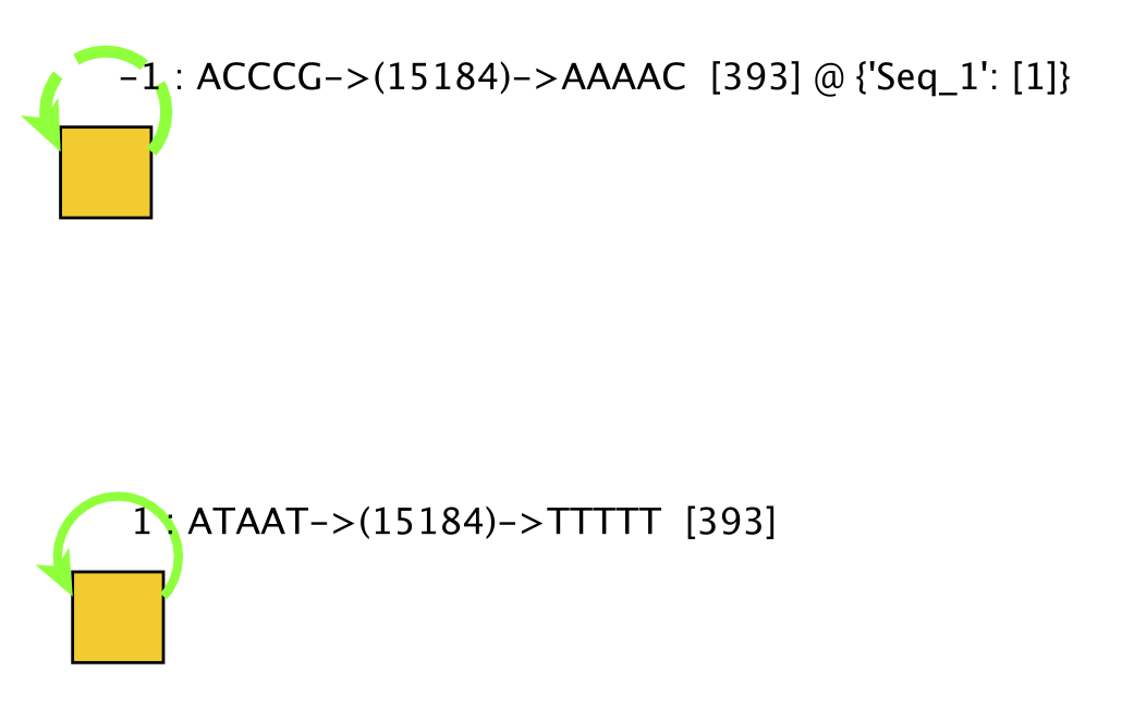
Figure 1: The .gml file contains a graph representation of the assembling¶

It can be visualized using the Yed program

The butterfly.mito.fasta file contains the produced sequence in fasta format. Most of the time you have a single contig corresponding to the complete sequence of the targeted genome. You can read this file using your favorite sequence/text editor or using the Unix cat command.

> cat butterfly.mito.fasta

>Seq_1 seq_length=15184; coverage=393.0; circular=True; -1 : ACCCG->(15184)->AAAAC  [393].{connection: 1}
ACCCGAAAATTTCCCAGAATAAATAAAATTTTACTAAACCTATCAACACCAAAAAACATT
TATATTTTTTTCCACTATTTATATAATTTTTAAAAAAAAAATATTTTTTAAAATTTAAAA
AAACACCCTCAGAGAAAATTCTCAAAAAAAAAAATCTTTTAAAGATAAAAAAGTTAATAA
ATTTCATTTAAATAAATTTTATTAGTAAATAATAAATATTAATAGATTAAATTAAATATT
AAATTATTAGGTGAAATTTTAATTTAATTAAAATTTTAATAAATAATATGATTTATTAAA
TTTTATAAAAAACTAGAATTAGATACTCTATTATTAAAAATTAAATAAAAAATACTAAAA
TAGTATATAATTATTTATAGAAACTTAAATAATTTGGCGGTATTTTAGTTCATTTAGAGG
AATCTGTTTAATAATTGATAATCCACGAATAAATTTACTTAATTTATATATTTTGTATAT
CGTTGTTAAAAAAATATTTTTTAATAAAAATAATATTTAAAAATTTTAAAATTAAATTAA
TTCAGATCAAGATGCAGATTATAATTAAGAATATAATGGATTACAATAAGAAATGATTAA
...
AGGGATTTCCTTTATATTTGGGGTATGAACCCAAAAGCTTATTTTAGCTTATTTTTAATT
TTATTTTTTTTTATTTATATAAATATTTATATGGAATGGTTTAGTAAAAAAATAAAAATA
TTATATAAATTATTAATAGTAAAAAAAAAATTAAGGTTTTTAAATTTTTTTAGTAATATA
TATATATATATATTAAAAATTTAATATATTAATATATTTAATAATATAATAAAAATATTT
AATTTATTAATATATAAATTAATATATTATAATTTTTTAGTTTTTAAAATTTTATATAGC
AATTTAGGTATTTAATATTTATTATGAAAAAAAAAAAAAAAAAAATTATTTAAGGGTTTA
ATAAGGGCCTAATAAAAAATTTTATAAAAGGGGATTTTTTTAAAAATTAAAAAATTTAAA
AAAC

Assembling a mitochondrion genome with the ORGanelle ASeMbler ¶

Step 1 : indexing the reads¶

Step 2 : Building the assembling graph¶

Step 3 : unfolding the graph to get the sequence¶

Table of Contents

Previous topic

Next topic

This Page

Assembling a mitochondrion genome with the ORGanelle ASeMbler¶

Step 1 : indexing the reads¶

Step 2 : Building the assembling graph¶

Step 3 : unfolding the graph to get the sequence¶

Assembling a mitochondrion genome with the ORGanelle ASeMbler ¶