The ORGanelle ASseMbler principles
Sequencing strategy: Low-coverage shotgun sequencing of genomic DNA
The resulting data of low-coverage shotgun sequencing of genomic DNA (gDNA), aka genome skimming, is the primary data used by ORG.asm. If we hypophethize that the organelle genomes represent several percent of the total gDNA (organellar genomes can be present in more than 1000 copies in a single cell), even with a modest depth of sequencing of the nuclear genome (around 1x coverage), on can hope to get more than 100x coverage for the organelle genomes and repeated regions (such as rDNA clusters). This allows the reconstruction of organelle genomes and repeated regions for up to 48 samples loaded in the same HiSeq 2500 lane.
For example, Consider that you sequence 3.10e6 pair-end reads -> 6.10e6 reads of 100bp
Organelle |
Chloroplast |
Mitochondria |
|---|---|---|
Belonging organelle |
5% |
0.5% |
Effective reads |
300,000 |
30,000 |
Base pairs |
30.10e6 |
3.10e6 |
Genome size |
150kb |
16Kb |
Sequencing depth |
200X |
187X |
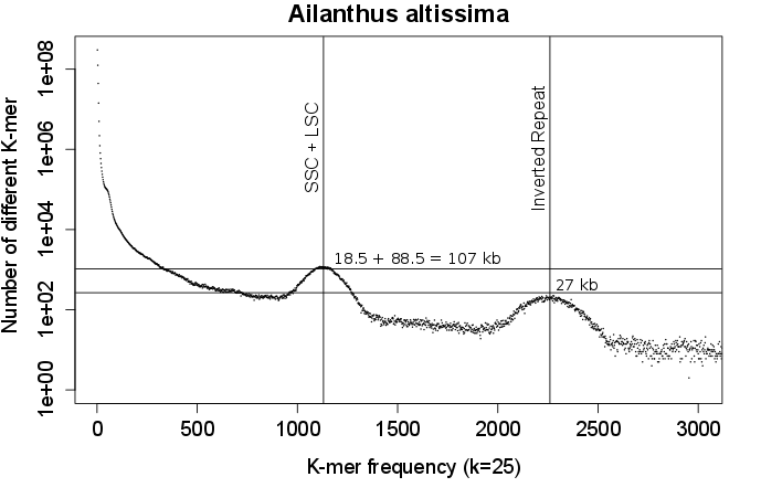
This can be further observed using the k-mer frequency spectrum of a plant genome low-coverage shotgun sequencing. The spectrum shows particular a shape with a high number of non-frequent kmer and a bimodal shape at intermediate and high frequency.
This shape can be explained by the mix of the low coverage sequencing the high coverage sequecing of the chloroplastic genome. Indeed the nuclear genome sequencing is responsible for a large number of unique or nearly unique k-mer and the high coverage sequencing of the chloroplastic genome translate into the bimodal distribution of moderatly and highly encountered k-mers, the bimodal distribution being due to the large duplicated region (Inverted Repeat) typical of the chloroplastic genome.
The assembly graph
The ORGanelle ASeMbler rely on a graph representation of the ongoing assembly. The graph used is what is called a De Bruijn graph but restricted to nodes representing substrings of a given length of the genome to reconstruct.
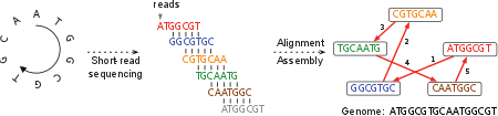
Figure 2: An example of the underlying graph (adapted from Compeau et al. (2011))
In our particular case, we work with words of the length of the reads produced by the shotgun sequencing. So the graph is also what is called a string graph for our set of reads (see Meyers (2005) for details).
The ORGanelle ASseMbler commands
Once installed, The ORGanelle ASeMbler enrich the command shell with the oa command. It is providing a set of sub-commands allowing for the complete assembling of small genomes (organelle genomes) from a genome skimming sequence dataset. You can have a basic idea on how to proced by following the tutorial.
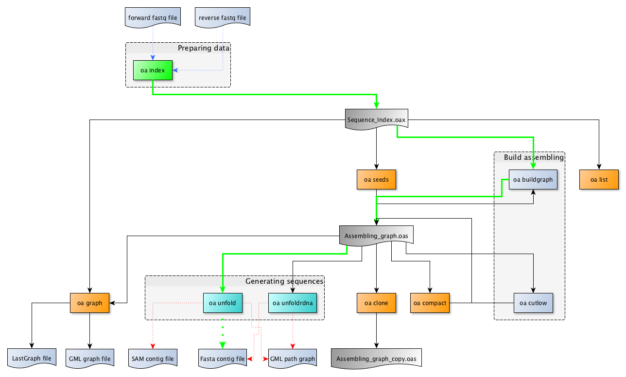
Figure 3: The organelle assembler’s provides a set of commands.
Several of these commands (at least three) have to executed to complete an assembling process.
The bold green path indicates the minimal succession of commands you need to run to assemble a sequence from a set of illumina reads.
The green dotted path indicates an alternative succession of commands commonly run to achieve the assembling process.
The fine blue dotted arrows indicate the data used by each of the commands.
The fine red dotted arrows indicate the final results provided by commands.
The orange boxed commands correspond to utility commands not required for the assembling but sometime useful to get or restore some information.
The set of sub-commands can be splitted in several categories corresponding to the main steps of the assembling procedure.
The file formats
Raw sequencing results (after adapter trimming) are usually provided in the fastq format, the raw result of the assembly in fasta format and the annotated result (with CDS, tRNA, …) in the EMBL format.